Documentation
A project made for The COVID-19 Detect & Protect Challenge
Index
1. Getting everything ready
1.1. Installing TensorFlow CPU
1.2. Installing TensorFlow GPU
2. Training your own model [OPTIONAL]
2.1. Giving birth to a new dataset
2.2. Cleaning and labeling your dataset
2.3. Starting the neural network training
2.4. Optimizing the training
3. Using the trained model
3.1. COVIDEO: Our implementation
3.1.1. Proximity detection: how does it work?
3.1.2. Tracking: how does it work?
3.1.2.1. Code explanation
3.1.3. Code of the desktop application
4. COVIDEO: a versatile model
5. Test COVIDEO online
6. Links list
1. Getting everything ready
These steps are necessary both if you want to train your own neural network or use the ones we provide here: (Faster RCNN & SSD Lite)[1].
It is important to stick with the software versions we recommend in this document, because newer versions may not work properly.
The first thing you will need to do is install the latest version of Python on your machine, following this link[2]. Remember to check the box “Add Python to PATH” before the installation begins.
Once you are done installing Python, you will need to get TensorFlow, either CPU or GPU (if you have an Nvidia GTX 650 or newer): if you do not know which one to choose, consider that TensorFlow CPU is much slower than its GPU version, so you should stick with the latter unless your machine does not have the requirements.
Before proceeding, you should install the latest version of Anaconda following this link[3], remembering to check the box “Add Anaconda to my PATH environment variable”. Once the installation is complete, open a new terminal window and type the following command:
conda create -n virtual_env pip python
The above will create a virtual environment that you will need to activate every time you want to work with TensorFlow (we will cover this).
1.1. Installing TensorFlow CPU
Open a new terminal window (if you have not done so already) and type the following commands:
                                activate virtual_env

                                pip install --upgrade tensorflow==1.15
Good news: you are done already! You can move forward.
1.2. Installing TensorFlow GPU
The installation of TensorFlow’s GPU version is much longer, but surely worth the effort!
Before proceeding, you should download the following packages:
CUDA Toolkit v10.0: link[4]
CuDNN v7.6.5 (Nov 5, 2019) for CUDA 10.0: link[5]
Let us install them!
CUDA is very easy to install (just run the executable file); CuDNN requires a little more effort: you will first need to follow the link provided above and create a user profile, if you do not have one already. Once you have logged in, download the package and extract the contents of the zip file (the folder named “cuda”) into INSTALL_PATH\NVIDIA GPU Computing Toolkit\CUDA\v10.0\, where INSTALL_PATH points to the installation directory specified during the installation of the CUDA Toolkit. By default, INSTALL_PATH = C:\Program Files.
There is still one thing left to do before installing TensorFlow GPU: setting up the necessary environment variables.
Go to Start and Search “environment variables”;
Click “Edit the system environment variables”: this should open the “System Properties” window;
In the opened window, click the “Environment Variables…” button to open the “Environment Variables” window;
Under “System variables”, search for and click on the “Path” system variable, then click “Edit…”;
Add the following paths, then click “OK” recursively to save the changes:
INSTALL_PATH\NVIDIA GPU Computing Toolkit\CUDA\v10.0\bin
INSTALL_PATH\NVIDIA GPU Computing Toolkit\CUDA\v10.0\libnvvp
INSTALL_PATH\NVIDIA GPU Computing Toolkit\CUDA\v10.0\extras\CUPTI\libx64
INSTALL_PATH\NVIDIA GPU Computing Toolkit\CUDA\v10.0\cuda\bin
You can now install TensorFlow GPU!
Open a new terminal window (if you have not done so already) and type the following commands:
                                activate virtual_env

                                pip install --upgrade tensorflow-gpu==1.15
You are all set!
You can now run our model or create your own.
The following section is optional, meaning you should only consider it if you want to train your own model.
2. Training your own model [OPTIONAL]
Before describing the actions that you will need to perform in order to start training your own model, we should first consider getting your virtual environment ready.
Open a new terminal window with virtual_env activated (if you have not done so already) and type the following command:
conda install pillow, lxml, jupyter, matplotlib, opencv, cython
The above command will install some packages in your virtual environment, allowing you to have all the most useful tools while training a neural network of such kind.
Now you will need to create the folder C:\Users\USER\Documents\TensorFlow (that we will call PATH_TO_TF), create another folder named “models” inside of it, download the TensorFlow Models from this link[6] and unzip the content directly into the models folder. This action will grant you access to a large variety of template models to choose from when training your own.
Rename the folder “models-r.1.13.0” into “models”.
The TensorFlow APIs use Protobufs to configure models and training parameters. Before the framework can be used, the Protobuf libraries must be downloaded and compiled.
Proceed as follows:
Head to the protoc releases page[7];
Download the latest release of protoc and extract the contents into a directory PATH_TO_PB of your choice;
Add PATH_TO_PB to your “Path” environment variable (like you did previously in section 2.2);
Open a new terminal window (it is necessary to close all the open ones before) and run the following command:
protoc PATH_TO_TF\models\research\object_detection\protos\*.proto --python_out=.
Once the above has completed, run the following command:
protoc PATH_TO_TF\models\research\object_detection\protos\*.proto --python_out=.
Now it is time to add all the necessary environment variables.
Just like you did previously, open the “Environment Variables” window:
Under “System variables”, search for and click on the “PYTHONPATH” system variable (see below);
If it does not exist, click “New…”, under “Variable name” type “PYTHONPATH” and under “Variable value” enter “PATH_TO_TF\models\research\slim”;
If it does exist, click “Edit” and add “PATH_TO_TF\models\research\slim” to the list;
Click “OK” recursively to save the changes.
You have completed all the steps required to set up your machine!
2.1. Giving birth to a new dataset
The first thing we need in order to train such a neural network is a set of images.
What kind of images and how many of them, anyways? There is never a golden number when it comes to neural networks.
Having to rely on our common sense, we found out that fifteen thousand images could do the trick, portraying about twenty thousand people wearing a face mask and twenty thousand people with a bare face. Diversity is the key to choosing a proper set of images: people must be carefully selected to be of different ethnicities, facial-features and ages, as well as to be portrayed both in close-ups and long shots.
2.2. Cleaning and labeling your dataset
The images do not contain information about the coordinates of the portrayed faces in a native way, so it is necessary to proceed with the dataset labeling operations. This procedure consists in labeling every masked and bare face present in each image, creating XML files that include the coordinates of the boxes identifying the faces and the corresponding classes (with mask or without mask).
In order to successfully perform this operation, a specific image-labeling software has been used: labelImg[8]. This software returns XML files in a PascalVOC format that will be used later in the process.
If we want to speed up the labeling process and we have a pre-trained model, we could perform an automatic pre-labeling operation: this action can be easily done with the script FaceDetectorXML.py[9], which is able to detect faces (either masked or bare) through a pre-trained model and to create XML files in accordance to the format used by labelImg.
It is worth remembering that manually checking annotations with labelImg and eventually correct them is highly recommended, as the human eye is much more precise than a pre-trained model’s.
Either way, images that did not contain faces were deleted at the end of the process.
2.3. Starting the neural network training
Once the labels have been assigned to the dataset, you can start performing the preliminary actions needed to set up your training environment: you will need both the images of the dataset in a PATH_TO_IMAGES folder and the XML files generated whilst labeling.
The first thing you need to do is dividing your XML files in two distinct folders: one folder PATH_TO_TRAIN_FOLDER will contain approximately 9/10 of the XMLs, another one PATH_TO_TEST_FOLDER will contain the remaining part. This division will allow TensorFlow to perform a successful training, using one portion of the dataset for training and one for testing.
The next steps will require you to create a folder PATH_TO_DATA and download two scripts into a separate PATH_TO_SCRIPTS folder: xml_to_csv[10] and generate_tfrecords[11]. They will first transform your XMLs into CSVs, then the resulting CSVs into TFRecords.
Open a new terminal window with virtual_env activated (if you have not done so already) and run the scripts as follows:
                                python PATH_TO_SCRIPTS\xml_to_csv.py -i PATH_TO_TRAIN_FOLDER -o PATH_TO_DATA\train_labels.csv


                                python PATH_TO_SCRIPTS\xml_to_csv.py -i PATH_TO_TEST_FOLDER -o PATH_TO_DATA\test_labels.csv


                                python PATH_TO_SCRIPTS\generate_tfrecords.py --label0=LABEL_0* --label1=LABEL_1* --csv_input=PATH_TO_DATA\train_labels.csv --img_path=PATH_TO_IMAGES --output_path=PATH_TO_DATA\train.record


                                python PATH_TO_SCRIPTS\generate_tfrecords.py --label0=LABEL_0* --label1=LABEL_1* --csv_input=PATH_TO_DATA\test_labels.csv --img_path=PATH_TO_IMAGES --output_path=PATH_TO_DATA\test.record
LABEL_0 and LABEL_1 are the labels used whilst labeling your dataset: the order does not matter, as long as you stick with it in the future.
The last things you need to do before starting the neural network training are the following:
Create a folder PATH_TO_CONFIG;
Create a new file inside PATH_TO_CONFIG named label_map.pbtxt and fill it with the following lines:
                                item {

                                 id: 1

                                 name: 'LABEL_0'

                                }

                                item {

                                 id: 2

                                 name: 'LABEL_1'

                                }

                                ;
Go to PATH_TO_TF\models\research\object_detection\samples\configs, pick a model of your choice and copy the config file into PATH_TO_CONFIG (the choice is really important, because some networks are more precise while others are faster – we trained both faster_rcnn_inception_v2_pets and ssd_mobilenet_v2_coco, because we believed that they could offer what we needed in terms of precision and performance);
Download the model corresponding to your choice from here[12], unzip it in PATH_TO_DATA and rename the model folder (e.g. “faster_rcnn_inception_v2_coco_2018_01_28”) into “ckpt_model”;
Make the following changes to the newly copied config file (lines are given with respect to faster_rcnn_inception_v2_pets.config and may change within other config files):
                                Line 9 Change num_classes to 2

                                Line 106 Change fine_tune_checkpoint to PATH_TO_DATA\ckpt_model\model.ckpt

                                Lines 125, 137 Change label_map_path to PATH_TO_CONFIG\label_map.pbtxt

                                Line 123 Change input_path to PATH_TO_DATA\train.record

                                Line 135 Change input_path to PATH_TO_DATA\test.record

                                Line 130 Change num_examples to the number of elements contained in PATH_TO_TEST_FOLDER
Be careful: it may be necessary to modify the initial_learning_rate (line 90) and the num_step (line 113) values for the training to work better. Indications on how to understand whether a neural network has been properly trained will be given in the “Optimizing the training” section.
This is great: you are ready to start your training!
Open a new terminal window with virtual_env activated (if you have not done so already) and type the following command:
python PATH_TO_TF\models\research\object_detection\legacy\train.py --logtostderr -- train_dir=PATH_TO_DATA\training\ -- pipeline_config_path=PATH_TO_CONFIG\CHOSEN_CONFIG_FILE.config
The training has finally started. After the initialization (that may take some time) you should see something like this:
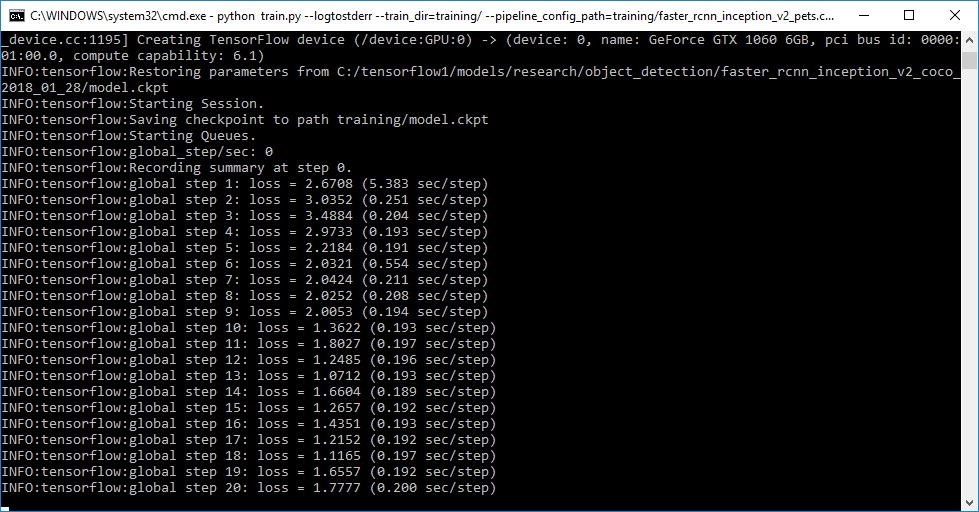
It is possible to monitor the evolution of the training opening a new terminal window with virtual_env activated, executing the following command and opening your localhost page from port 8080[13]:
tensorboard --logdir=PATH_TO_DATA\training\ --host localhost --port 8088
When the training is done, you can proceed exporting the model.
In a terminal window with virtual_env activated, run the following command:
python PATH_TO_TF\models\research\object_detection\export_inference_graph.py --input_type image_tensor --pipeline_config_path PATH_TO_CONFIG\CHOSEN_CONFIG_FILE.config --trained_checkpoint_prefix PATH_TO_DATA\training\model.ckpt-XXXXXX --output_directory PATH_TO_DATA\inference_graph\
Replace XXXXXX with the highest-numbered ckpt file present in PATH_TO_DATA\training\
2.4. Optimizing the training
The tensorboard’s loss charts should look something like this:
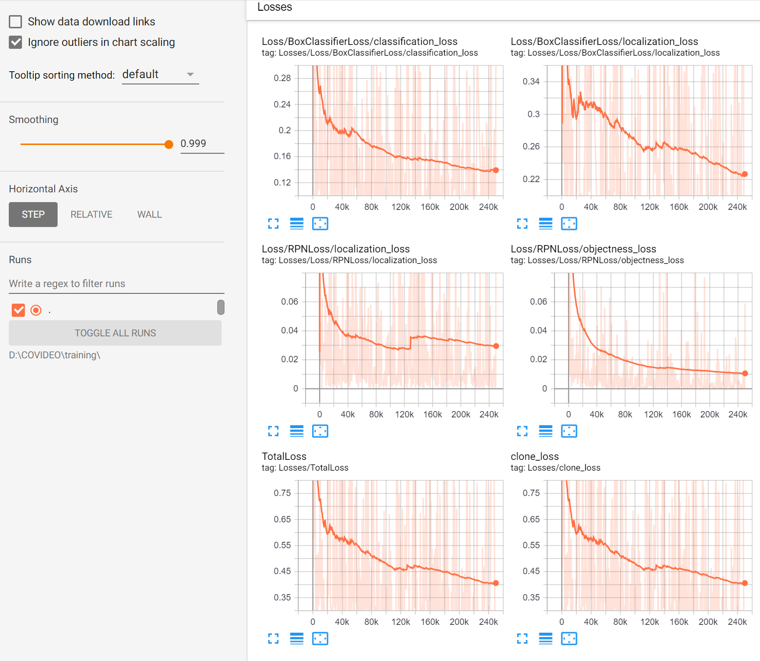
If your charts differ a lot from these, it may have something to do with the learning rate used during the training.
The picture shown below describes all the possible cases:
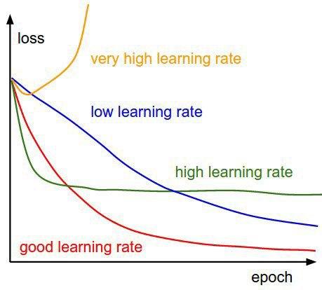
If the curves resemble the green or blue lines, we recommend multiplying or dividing the current learning rate by 10 and adjusting the number of steps accordingly.
3. Using the trained model
Once our model has been properly trained, it is time to exploit its full potential.
We thought it would be useful to estimate the global adhesion to the recently introduced sanitary laws, keeping count of the people that wear a mask and compare it to the number of people who do not. This can be achieved interfacing the software we provide[14] with a video feed, originated from a webcam or a surveillance camera, but also from a video file.
The applications of this trained model, however, are countless: we will illustrate some of the possible implementations at the end of this section.
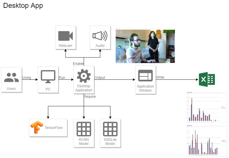
3.1. COVIDEO: Our implementation
Once the archive containing our software has been downloaded, the content has to be extracted in a APPLICATION_PATH folder in order to be executed.
The software is plug and play, meaning it can be directly executed on a machine that has been configured following our guide. The only step required in order to execute the application, at this point, is to install all the needed libraries. In a terminal window with virtual_env activated, run the following command:
pip install xlsxwriter playsound pyqt5 scipy numpy
You are all set! :)
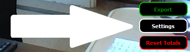
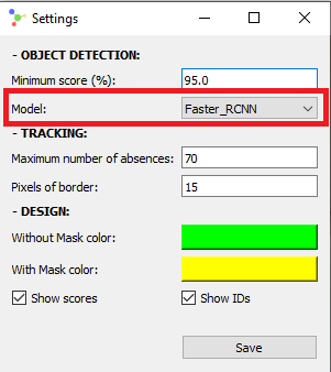
It is worth noticing that the application uses the Faster RCNN model by default, which requires high computational resources (a proper GPU unit) in order to work smoothly. If the application seems to be running slowly (or the results are not as expected), the model can be switched manually to SSD Lite from the settings menu (white button in the lower right corner):
Although the default input is the system webcam, it is possible to change it to a chosen video replacing the line 419 as follows:
Old:
self.video = cv2.VideoCapture(0)
New:
self.video = cv2.VideoCapture(PATH_TO_VIDEO)
In a terminal window with virtual_env activated, run the following commands:
                                cd APPLICATION_PATH\DesktopApp\


                                python app.py
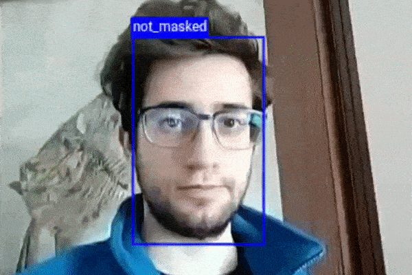
Once the initialization process has been completed, a window similar to the one illustrated in the introduction section will pop up.
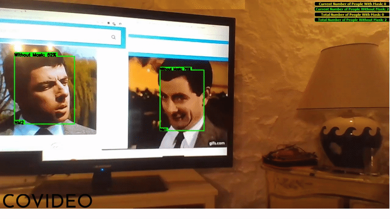
The user interface shows a box around every detected face, providing the confidence value (as a percentage) and the class of the detection ("M" if the person wears a mask, "NM" if not). If two people (of whom at least one is not wearing a face mask) keep a distance between each other lower than one meter for one consecutive second or more, an alarms goes off and the two people's boxes become red, reminding people to respect precautionary distances.
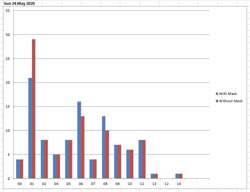
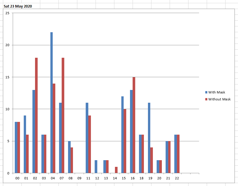
When the application is closed, the total counts (displayed in the upper right corner) are saved as a temporary file in C:\Users\USER\AppData\Local\Temp\: this will allow the application to load the previously saved total counts on the next startup.
It is possible to manually reset total counts by clicking the red button in the lower right corner, as well as to export data into a file by clicking the green button. The exported file displays data in a user-friendly manner, giving interesting visual information about the behavior of people throughout the days of the week, as showed in the pictures below:
The complete code of the desktop application is provided at the end of this section.
3.1.1. Proximity detection: how does it work?
Since we can rely on a bidimensional space only, we cannot compute distances between people with triangulation operations: we have to think of a smarter approach.
The easiest way for a machine to compute distances in a non-tridimensional space is an obect-related approach. What does this mean? People that are closer to the camera will have relatively bigger bidimensional faces than people that are far from it, so it does not make any sense to calculate Euclidian distances between them: we can only assume that they are not standing much close to each other. On the other hand, if people are standing at the same camera-related depth level, they will have faces of comparable sizes. Only in this case Euclidian distances are calculated, making the most out of data that we can easily access: if there is enough space for a certain number of faces to be placed between two people, they must be standing relatively far from each other.
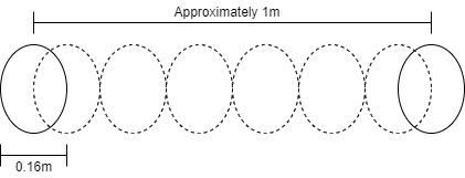
Considering that a normal face is around 16 centimeters wide, a good number of units to guarantee a distance of one meter between people is 1 / 0.16 = 6.
The proximity detection algorithm code is quite self-explanatory, but we kindly invite the reader to refer to section 3.1.2 should they have trouble understanding it. We preferred to explain Euclidian distances and to provide a better view of the overall application in a more proper context, in order not to repeat ourselves.
This is the code used for detecting proximity:
                                # function that receives the model output.

                                # masked and not_masked are two dictionaries

                                # having the ID of each face (masked or bare) as

                                # keys, the coordinates of the boxes containing the

                                # faces as values (i.e. ID 3 => [0, 200, 0, 200]).

                                # coordinates are expressed as [xmin, xmax, ymin, ymax].

                                def proximity_detector(masked, not_masked):

                                 result = set()

                                 std_ratio = 2 / 3 # standard parameter

                                 std_face_width = 0.16 # standard face width in meters


                                 # is there anyone that does not have a mask? If yes, verify that no one is close to him!

                                 for item in not_masked.items():

                                  first_width = item[1][1] - item[1][0]

                                  first_height = item[1][3] - item[1][2]

                                  first_max = max(first_width, first_height)

                                  first = (item[1][0] + first_width / 2, item[1][2] + first_height / 2) # x,y coordinates of NM's centroid


                                  # are there any masked people close to the one who's not masked?

                                  for m in masked.items():

                                   second_width = m[1][1] - m[1][0]

                                   second_height = m[1][3] - m[1][2]

                                   second_max = max(second_width, second_height)

                                   second = (m[1][0] + second_width / 2, m[1][2] + second_height / 2) # x,y coordinates of M's centroid

                                   if (first_max <= second_max and first_max > second_max * std_ratio) or\

                                    (second_max < first_max and second_max > first_max * std_ratio): # are the faces' depths comparable?

                                    distance = math.sqrt((first[0] - second[0])**2 + (first[1] - second[1])**2)

                                    if distance / ((first_max + second_max) / 2) < 1 / std_face_width: # people are too close to each other!

                                     result.add(tuple(sorted(('NM{}'.format(item[0]), 'M{}'.format(m[0]))))) # tuple+sorted combo is for preventing simmetries


                                  # are there any unmasked people close to the one who's not masked?

                                  for nm in not_masked.items():

                                   if nm[0] != item[0]:

                                    second_width = nm[1][1] - nm[1][0]

                                    second_height = nm[1][3] - nm[1][2]

                                    second_max = max(second_width, second_height)

                                    second = (nm[1][0] + second_width / 2, nm[1][2] + second_height / 2) # x,y coordinates of M's centroid

                                    if (first_max <= second_max and first_max > second_max * std_ratio) or\

                                     (second_max < first_max and second_max > first_max * std_ratio): # are the faces' depths comparable?

                                     distance = math.sqrt((first[0] - second[0])**2 + (first[1] - second[1])**2)

                                     if distance / ((first_max + second_max) / 2) < 1 / std_face_width: # people are too close to each other!


                                      result.add(tuple(sorted(('NM{}'.format(item[0]), 'NM{}'.format(nm[0]))))) # tuple+sorted combo is for preventing simmetries


                                 return result
3.1.2. Tracking: how does it work?
If we want to count the number of people that are recorded in a portion of time, it is necessary to make sure that multiple detections related to the same person are associated to a single individual: faces must be tracked not to lose associations.
We decided to base our tracking algorithm on the Euclidian distance between the faces’centroids.
What does it mean? The detection model’ s output is, for each frame, a set of coordinates describing the eventual faces’ positions.
Given these coordinates, it is possible to compute the centroids (the coordinates of the center of each box).
Once a face centroid has been computed, it is possible to exploit its information to decide whether a face that is present in two frames (consecutive or not consecutive) belongs to the same person:
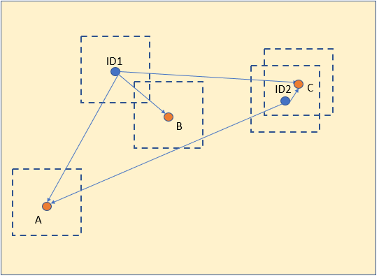
The blue dots are the box centroids of the n-th frame, while the orange ones are the box centroids of the (n+1)-th frame.
The Euclidian distance between ID1 and B is lower than both the other distances (ID1-A, ID2-C), so B is considered an update of ID1.
The same happens for ID2: C is considered an update of ID2 because it is the closest centroid amongst the new centroids.
As for centroid A, it will be assigned a new ID (and a new face consequently) because there is no eligible predecessor.
Let us consider the next couple of frames:
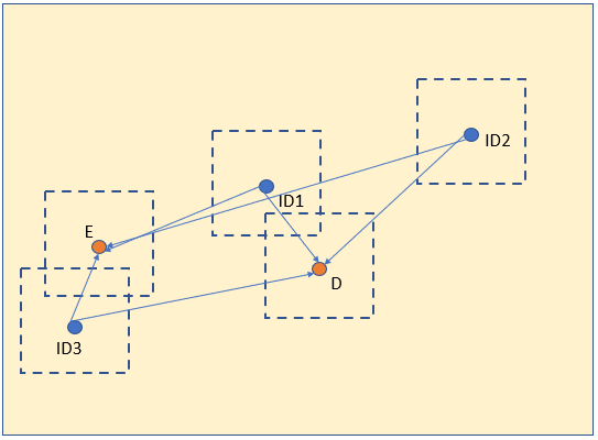
The Euclidian distance between ID1 and D is lower than distance between ID1 and E, so D is considered an update of ID1.
The same happens for ID3 and E, but what about the centroid ID2? It does not have any new candidate box, so it is not shown in the (n+2)-th frame.
If no unassigned new boxes are detected in a preset number of consecutive instants (absences) in ID2’s area of interest, ID2 will be discarded.
The mechanism described above is used in order to prevent possible instabilities to compromise results.
Another important aspect to be considered is the set of boundaries the frames are ideally made of:
When at least one corner of the box crosses the red line in a given frame and the box is not present in the very next frame, an assumption is made: the person moved away, so their ID is discarded. This behavior differs from the case illustrated through the previous images, as the ID is discarded without waiting a preset amount of time.
3.1.2.1. Code explanation
The first we need to do is import the necessary libraries:
                                import numpy as np

                                from scipy.spatial import distance as dist
Next comes the creation of the class Tracker.
- nextID is the box-associated IDs counter
- objects is the dictionary containing the centroids
- absences is the dictionary that keeps count of the absences for each box contained in
- coordinates is the dictionary containing the boxes’ coordinates
- coordinates_backup is an auxiliary dictionary
- maxAbsences is the maximum number of absences that is allowed before a box is discarded
                                class Tracker():

                                 def __init__(self, maxAbsences=50, startID=1):


                                  # ID Counter

                                  self.nextID = startID


                                  # To store current objects

                                  self.objects = {}


                                  # To count how many consecutive frames an object is absent

                                  self.absences = {}


                                  # To store coordinates to return

                                  self.coordinates={}


                                  # To backup

                                  self.coordinates_backup={}


                                  # Maximum number of consecutive absences of an object before its deletion

                                  self.maxAbsences = maxAbsences
It is necessary to have a method that adds new faces to track (method add):
                                 def add(self, centroid):

                                  # Add a new detected object and increases object counter

                                  self.objects[self.nextID] = centroid

                                  self.absences[self.nextID] = 0

                                  self.nextID += 1
The method remove allows to remove specific faces from the list of faces to be tracked:
                                 def remove(self, objectID):

                                  # Remove a disappeared object

                                  del self.objects[objectID]

                                  del self.absences[objectID]
The method refresh allows to update the faces’ centroids, but also to remove or add them by calling remove and add respectively:
                                 def refresh(self, inputObjects, imgSize, border):

                                  # If the list of input objects of the current frame is empty:

                                  if len(inputObjects) == 0:


                                   # It is necessary to add an absense to every object present in the archive

                                   for objectID in list(self.absences.keys()):

                                    self.absences[objectID] += 1


                                    # If an object is absent and in the last presence was at the boundaries of the picture

                                    # it will be deleted

                                    x_min, x_max, y_min, y_max = self.coordinates_backup[objectID]


                                    if ((x_min in range(-50,border))

                                     or (x_max in range(imgSize[1]-border,imgSize[1]+50))

                                     or (y_min in range(-50,border))

                                     or (y_max in range(imgSize[0]-border,imgSize[0]+50))):


                                     self.remove(objectID)

                                     del self.coordinates_backup[objectID]


                                    # If an object has reached the maximum number of consecutive absences, it is deleted

                                    elif self.absences[objectID] > self.maxAbsences:

                                     self.remove(objectID)

                                   self.coordinates={}

                                   return self.coordinates


                                  # Compute centroids for the objects in the current frame

                                  inputCentroids = [self.calc_centroid(inputObject) for inputObject in inputObjects]

                                  # if there are no objects in the archive, all the input objects are added

                                  if len(self.objects) == 0:

                                   for i in range(0, len(inputCentroids)):

                                    self.coordinates[self.nextID]=inputObjects[i]

                                    self.coordinates_backup[self.nextID]=inputObjects[i]

                                    self.add(inputCentroids[i])

                                  # else it necessary to match the input objects with the already existing ones

                                  else:

                                   objectIDs = list(self.objects.keys())

                                   objectCentroids = list(self.objects.values())


                                   # compute distances between input objects and the already existing ones

                                   D = dist.cdist(np.array(objectCentroids), np.asarray(inputCentroids))


                                   # Sort and match by distance

                                   rows = D.min(axis=1).argsort()

                                   cols = D.argmin(axis=1)[rows]


                                   usedRows = set()

                                   usedCols = set()


                                   for (row, col) in zip(rows, cols):

                                    # if (row,col) had already examined, ignore them

                                    if row in usedRows or col in usedCols:

                                     continue

                                    #else take for the current row the object ID and set its

                                    # updated centroid and reset its absences

                                    objectID = objectIDs[row]

                                    self.objects[objectID] = inputCentroids[col]

                                    self.coordinates[objectID]=inputObjects[col]

                                    self.coordinates_backup[objectID]=inputObjects[col]

                                    self.absences[objectID] = 0


                                    # add current col and row to the already used list

                                    usedRows.add(row)

                                    usedCols.add(col)


                                   # get the unused rows indexes (correspondent to objects that need

                                   # to be removed)

                                   unusedRows = set(range(0, D.shape[0])).difference(usedRows)

                                   #get the unused columns indexes (correspondent to the input objects

                                   #that need to be added)

                                   unusedCols = set(range(0, D.shape[1])).difference(usedCols)


                                   # if the number of input objects is equal or lower than the number of

                                   # objects in the archive, it means that some objects are absent

                                   if D.shape[0] >= D.shape[1]:

                                    for row in unusedRows:

                                     objectID = objectIDs[row]

                                     self.absences[objectID] += 1

                                     x_min, x_max, y_min, y_max = self.coordinates_backup[objectID]


                                     # if in the preview frame an absent object was at the

                                     #boundary of the image, it needs to be deleted from the archive

                                     # (object exiting from the picture)

                                     if ((x_min in range(-border*4,border))

                                      or (x_max in range(imgSize[1]-border,imgSize[1]+border*4))

                                      or (y_min in range(-border*4,border))

                                      or (y_max in range(imgSize[0]-border,imgSize[0]+border*4))):


                                      self.remove(objectID)

                                      del self.coordinates_backup[objectID]

                                      del self.coordinates[objectID]


                                     # an object has reached the maximum number of consecutive absenses

                                     # needs to be deleted

                                     elif self.absences[objectID] > self.maxAbsences:

                                      self.remove(objectID)

                                      if objectID in list(self.coordinates.keys()):

                                       del self.coordinates[objectID]


                                   # else if the number of input objects is greater than the number of

                                   #objects in the archive of objects, new objects need to be added

                                   else:

                                    for col in unusedCols:

                                     self.coordinates[self.nextID]=inputObjects[col]

                                     self.coordinates_backup[self.nextID]=inputObjects[col]

                                     self.add(inputCentroids[col])

                                  return self.coordinates


                                 def calc_centroid(self,detection):

                                  # calculate the centroid

                                  x_min, x_max, y_min, y_max = detection

                                  return [int((x_min+x_max)/2.0),int((y_min+y_max)/2.0)]


                                 def reset(self):

                                  self.nextID = 1

                                  self.objects = {}

                                  self.absences = {}

                                  self.coordinates={}
3.1.3. Code of the desktop application
The link is provided in the attachments of the project.
You can also download it from here[15].
4. COVIDEO: a versatile model
Someone might not be interested in consulting any kind of statistics about the number of people wearing face masks: they might want to control access to their premises or guarantee strict safety policies.
COVIDEO adapts to any situation where an automatic system can replace expensive manual screening activities.
Let us suppose a public transport company wants to assure that everyone who uses the subway wears a face mask: a standard surveillance camera can be placed at the entrance of the subway station and connected to a COVIDEO application. The application instructs specific doors to open only when certain conditions are met (persons wear a face mask). The idea can be applied to every premise that is able to guarantee the entrance of a person at a time: subway stations, airports, restaurants, shops, etc.
Let us now suppose Mario owns a grocery store where affluence is considerably high: he would like to guarantee his clients that people meticulously observe safety measures in his store. Mario installs a surveillance camera at the entrance and connects it to an application similar to the one we developed: clients are asked to wear a face mask before entering the store and, most importantly, are reassured that 99.9% of clients that accessed the store in the last two weeks were wearing a face mask.
In general, COVIDEO aims to help people live without the fear of social relations. As humans, we need to live in connection with each other in order to live a healthy life: we will not let anything stand between us and the need for social interactions.
5. Test COVIDEO online

In order to give the possibility to test COVIDEO to everyone, we decided to create a website hosting some demos: this system allows to test the neural network simply accessing a website through a web browser.
The website's demo pages make use of Tensorflow JS APIs and the trained neural network models to process the images uploaded by the user, or the webcam video feed.
The original models have been converted to Tensorflow JS-compatible models with the following command:
tensorflowjs_converter --input_format=tf_saved_model --output_format=tfjs_graph_model --signature_name=serving_default --saved_model_tags=serve PATH_INPUT_MODELS PATH_OUTPUT_MODELS
Since the processing times of the Faster RCNN Inception v2 network are too slow to handle a real-time video source (with the network being computationally expensive itself), we decided to train a dedicated network with the same dataset.
The SSDLite Mobilenet v2 model has been used for this purpose, a faster solution that loses precision.
Both the neural networks can be tested in the website's demo pages, except for the "Webcam Live" option that allows the use of the SSDLite Mobilenet v2 network only.
- Google Chrome Versione 81.0.4044.138 (Official build) (a 64 bit)
- Firefox 76.0.1 (64 bit)
- Microsoft Edge 44.18362.449.0
The exceptionally low processing times of the SSDLite Mobilenet v2 network brought us to consider the creation of a webview-based Android mobile app, extending the system's usability and demonstrating the results' quality, even with mobile devices.
The app has been tested on the following devices:- Redmi Note 7
- Huawei Mediapad M5 Lite
- Android 7.0 (Nougat)
- Android 7.1.1 (Nougat)
- Android 8.0 (Oreo)
- Android 9.0 (Pie)
- Android 10.0 (Q)
6. Links list
[1]: https://www.covideo.it/uploads/Faster_RCNN.pb & https://www.covideo.it/uploads/SSD_lite.pb
[2]: https://www.python.org/downloads/
[3]: https://www.anaconda.com/products/individual#windows
[4]: https://developer.nvidia.com/cuda-10.0-download-archive
[5]: https://developer.nvidia.com/rdp/cudnn-download
[6]: https://github.com/tensorflow/models
[7]: https://github.com/protocolbuffers/protobuf/releases/
[8]: https://pypi.org/project/labelImg/
[9]: https://www.covideo.it/uploads/FaceDetectorXML.py
[10]: https://github.com/EdjeElectronics/TensorFlow-Object-Detection-API-Tutorial-Train-Multiple-Objects-Windows-10/blob/master/xml_to_csv.py
[11]: https://github.com/EdjeElectronics/TensorFlow-Object-Detection-API-Tutorial-Train-Multiple-Objects-Windows-10/blob/master/generate_tfrecord.py
[12]: https://github.com/tensorflow/models/blob/master/research/object_detection/g3doc/detection_model_zoo.md
[13]: http://localhost:8088/
[14]: https://www.covideo.it/uploads/DesktopApp.zip
[15]: https://www.covideo.it/uploads/app.py
[16]: https://www.covideo.it/uploads/COVIDEO.apk